线性代数

标量

x = torch.tensor(3.0)
y = torch.tensor(2.0)
x + y, x * y, x / y, x**y

(tensor(5.), tensor(6.), tensor(1.5000), tensor(9.))

向量

你可以将向量视为标量值组成的列表，可以通过张量的索引来访问任一元素

x = torch.arange(3)
x

tensor([0, 1, 2])

x[2]

tensor(2)

len(x)

3

x.shape

torch.Size([3])

A = torch.arange(6).reshape(3, 2)
A

tensor([[0, 1],
        [2, 3],
        [4, 5]])

矩阵的转置，对称矩阵等于其转置

A.T

tensor([[0, 2, 4],
        [1, 3, 5]])

就像向量是标量的推广，矩阵是向量的推广一样，我们也可以构建具有更多轴的数据结构

a = 2
X = torch.arange(24).reshape(2, 3, 4)
a + X, (a * X).shape

(tensor([[[ 2,  3,  4,  5],
          [ 6,  7,  8,  9],
          [10, 11, 12, 13]],
 
         [[14, 15, 16, 17],
          [18, 19, 20, 21],
          [22, 23, 24, 25]]]),
 torch.Size([2, 3, 4]))

给定具有相同形状的任何两个张量，任何按元素二元运算的结果都是具有相同形状的张量

A = torch.arange(6, dtype=torch.float32).reshape(2, 3)
B = A.clone()
A, A + B

(tensor([[0., 1., 2.],
         [3., 4., 5.]]),
 tensor([[ 0.,  2.,  4.],
         [ 6.,  8., 10.]]))

两个矩阵的按元素乘法称为哈达玛积(Hadamard product)

A*B
tensor([[ 0.,  1.,  4.],
        [ 9., 16., 25.]])

计算其元素的和

x = torch.arange(3, dtype=torch.float32)
x, x.sum()

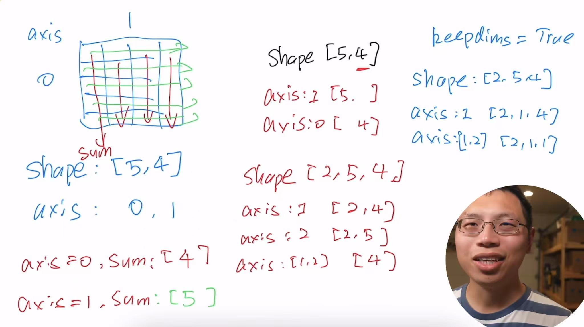
(tensor([0., 1., 2.]), tensor(3.))

指定求和汇总张量的轴

A.shape, A.sum(axis=0).shape,A.sum(axis=0)

(torch.Size([2, 3]), torch.Size([3]), tensor([3., 5., 7.]))
A.shape, A.sum(axis=1).shape

A.shape, A.sum(axis=1).shape,A.sum(axis=1)

(torch.Size([2, 3]), torch.Size([2]), tensor([ 3., 12.]))

 A.sum(axis=[0,1]),A.sum(axis=[0, 1]) == A.sum()

 (tensor(15.), tensor(True))

一个与求和相关的量是平均值

A.mean(), A.sum() / A.numel()

(tensor(2.5000), tensor(2.5000))

A.mean(axis=0), A.sum(axis=0) / A.shape[0]

(tensor([1.5000, 2.5000, 3.5000]), tensor([1.5000, 2.5000, 3.5000]))

A.mean(axis=1), A.sum(axis=1) / A.shape[1]

(tensor([1., 4.]), tensor([1., 4.]))

计算总和或均值时保持轴数不变（一个三维的矩阵，按一个维度求和，变成一个二维的矩阵；一个二维的矩阵，按一个维度求和，变成一个一维的向量，但是我们不想丢掉这个维度）

sum_A = A.sum(axis=1, keepdims=True)
sum_A, sum_A.shape,A.sum(axis=1)

(tensor([[ 3.],
         [12.]]),
 torch.Size([2, 1]),
 tensor([ 3., 12.]))

通过广播将A除以sum_A（维度必须是一样的）

A / sum_A

tensor([[0.0000, 0.3333, 0.6667],
        [0.2500, 0.3333, 0.4167]])

某个轴计算A元素的累积总和

A.cumsum(axis=0),A.cumsum(axis=1)

(tensor([[0., 1., 2.],
         [3., 5., 7.]]),
 tensor([[ 0.,  1.,  3.],
         [ 3.,  7., 12.]]))

点积是相同位置的按元素乘积的和 torch.dot只能用于一维向量

y = torch.ones(3, dtype = torch.float32)
x, y, torch.dot(x, y)

(tensor([0., 1., 2.]), tensor([1., 1., 1.]), tensor(3.))

我们可以通过执行按元素乘法，然后进行求和来表示两个向量的点积

torch.sum(x * y)

tensor(3.)

矩阵向量积是一个长度为的列向量，其元素是点积

A.shape, x.shape, torch.mv(A, x), A@x 

(torch.Size([2, 3]), torch.Size([3]), tensor([ 5., 14.]), tensor([ 5., 14.]))

我们可以将矩阵-矩阵乘法看作是简单地执行次矩阵向量积，并将结果拼接在一起，形成一个矩阵

B = torch.ones(3,3)
torch.mm(A,B)

tensor([[ 3.,  3.,  3.],
        [12., 12., 12.]])

范数是向量元素平方和的平方根：$$|\mathbf{x}|2 = \sqrt{\sum^n x_i^2}$$

u = torch.tensor([3.0, -4.0])
torch.norm(u)

tensor(5.)

范数是向量元素平方和的平方根：$$|\mathbf{x}|1 = \sum^n |x_i|$$

torch.abs(u).sum()

tensor(7.)

矩阵的弗罗贝尼乌斯范数（Frobenius norm）是矩阵元素的平方和的平方根：$$|\mathbf{x}|F = \sqrt{\sum^n\sum_{j=1}^n x_{ij}^2}$$

torch.norm(torch.ones((4, 9)))

tensor(6.)

标量 ​

向量 ​

标量

向量